RF fab-model test coupons¶
Test coupons measure what the board house actually builds (dielectric constant and loss, heights, copper thickness, etch, roughness, solder mask) so that an RF design starts from measured values instead of the fab’s nominal stackup. You order the coupon boards with the same options as the product, measure them with a two-port VNA, and run one command that fits the fab parameters, with uncertainties, and writes an updated stackup for yapnr’s models.
The design, with its reasoning and references, is design/rf-fab-coupons.md (issue #32). This page is the user guide: what to order, how to measure, how to run the extraction and how its results feed back. Nothing has been ordered or measured yet; every number below comes from models and synthetic measurements.
What is in the repository¶
Path |
Contents |
|---|---|
board A (4 layers): KiCad project, catalogue, expected S-parameters, fab |
|
board B (6 layers, stripline): the same |
|
board O, the OSH Park Order 0 uploads O0-M, O0-W, O0-D |
|
Order 0: the boards, the pre-registration, the predictions |
|
the layout of a measurement session |
|
|
generator, models, calibration, fit, synthetic sessions (numpy only) |
|
the 2D cross-section tables of each stackup’s line families |
All commands below are python -m yapnr.rf.coupons <command> from a checkout (numpy and PyYAML
are the only dependencies), or bazel run //yapnr/rf/coupons:cli -- <command>.
1. The boards¶
Board |
Stackup |
Lines |
Panel (mm) |
|---|---|---|---|
A |
JLCPCB JLC04161H-7628, 4L |
L1 grounded coplanar (P) and microstrip (M), masked |
176 × 182 |
B |
JLCPCB JLC06161H-2116C, 6L |
L3 stripline (S) between L2 and L4; L1 P tie set |
224 × 120 |
O |
OSH Park 4L, FR408HR |
Order 0: L1 microstrip M (over In1) and W (over L4) |
three uploads, below |
Every structure is a stick: a 15 mm (or wider) strip of board with an edge SMA at each end, held in the panel by mouse-bite tabs on its long sides. The 50 Ω lines are P 0.291 mm with 0.20 mm gaps (L1, under mask) and M 0.348 mm (L1, under mask) on board A; board B, on the product’s JLC06161H-2116C, has S 0.279 mm (L3) and P 0.350 mm with 0.20 mm gaps. Each board has
a multiline TRL set of its main family: thru (20 mm) and lines of 2.5, 6.5, 16, 40 and 100 mm more, a reflect (via shorts at the reference planes) and a 28 mm verification line;
variants over 40 mm: the line at 0.7 and 1.4 times its width, with the mask opened, and (board A) microstrip with and without mask;
held-out structures the fit never sees: a directly fed ring (resonance notches at 2.9, 5.8 and 11.6 GHz; the two feed paths also cancel at 2.2, 6.5 and 10.9 GHz, which the check ignores), an open quarter-wave and a shorted half-wave stub (notches at 5.8 GHz), a λ/4 coupled-line section;
DC meanders on every copper layer (two widths, four-wire pads) and a 50-via chain;
a microsection stick with every line family side by side and a cut line.
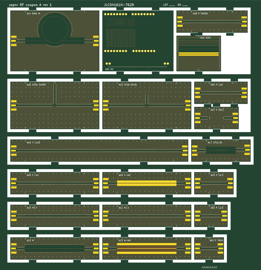
The full list is in each board’s catalog.json and in design §5. Board B is built on the
product’s stackup, JLC06161H-2116C (owner decision, 2026-10-02): its L1 dielectric is 2 × 2116, not
board A’s 7628, so board A’s fit is no longer a prior for it. The stripline alone measures the
mix of the core’s and the 2116’s εr but not the split; the L1 tie set (P under mask) and a
mask-off copy of the tie line (B24, P-MO) separate the mask from the 2116’s εr on board B itself.
The former board B on JLC06161H-7628, which shares board A’s L1 cross-section, stays defined (its
tables and the synthetic studies below use it): there, board B alone cannot split the core’s and
the 7628’s εr (correlated −0.97 to −1.00), and board A’s fit as the prior (--prior <board A>/fit.json, §4) cut the core’s εr σ from 0.14 to 0.05 and the 7628’s from 0.09 to 0.03 in a
synthetic test.
Regenerating¶
YAPNR_KICAD_CLI=<headless kicad-cli> python -m yapnr.rf.coupons generate \
    --stackup JLC04161H-7628 --out examples/rf-coupons/JLC04161H-7628
python -m yapnr.rf.coupons expected --stackup JLC04161H-7628 \
    --out examples/rf-coupons/JLC04161H-7628/expected
generate writes the KiCad project (stackup set in the board setup, zones left unfilled), runs
KiCad’s DRC with the zones refilled (the boards are DRC-clean: no violations, no unconnected
items), exports Gerbers and Excellon drill files and packs them with the fab notes into
fab/board-<A|B>-fab.zip. Use the headless KiCad (DEVELOPERS.md), never the GUI bundle. The
generator is parametric in the stackup; a new stackup needs its 2D tables first (§6).
The OSH Park edge launch (Order 0)¶
The OSH Park 4-layer boards of Order 0 use the Cinch 142-0701-851 end-launch SMA (a 0.51 x 0.25 mm
flat tab contact) on every port, with a launch designed in 2D for each region
(yapnr/rf/coupons/launch.py, shipped as data/launch-oshpark-4l-fr408hr.json):
Region M (L1 microstrip over In1.Cu, 0.20 mm): a 0.80 mm grounded-coplanar pin pad from the 0.381 mm copper keep-back to 0.4 mm past the tab, its coplanar gap solved with the tab and a solder fillet on it (and solved again for the bare toe), In1.Cu cut out under the pad so it references In2.Cu; then a 1.2 mm taper to the line in which the cut-out closes at constant 2D impedance, and a 2 mm flare of the L1 ground to the line’s 1.0 mm keep-away.
Region W (L1 over B.Cu, inner layers removed): the same pad, then a coplanar taper to the 3 mm line whose gap follows the 50 Ω solution until the ground has to clear the line.
Ground: the manufacturer’s leg pads on F.Cu and B.Cu, vias inside and behind each pad, a row 0.7 mm from the edge, and fences (0.3 mm drill, 1.0 mm pitch) 0.50 mm outside the channel to 4 mm past the launch. The solder mask covers the pad’s gap (a web against bridges) and opens over the line and its keep-away from a 0.2 mm dam at the pad end.
python -m yapnr.rf.coupons.launch show                     # the numbers and the rule check
python -m yapnr.rf.coupons.launch design --region M        # re-solve (FEA environment)
YAPNR_KICAD_CLI=<headless kicad-cli> python -m yapnr.rf.coupons.launch board --region M --out <dir>
board writes a small check board (a thru and a line stick carrying the launch, OSH Park’s
4-layer design rules) and runs KiCad’s DRC on it. The launch is not 3D-tuned: the multiline
calibration removes it as long as it repeats. A 3D (openEMS) sweep should still check the 0.38 mm
of bare laminate under the tab at the milled edge, the connector’s set-back and the tab’s height
in the 1.73 mm slot, the solder fillet, the closing profile of the In1.Cu cut-out and the return
path through the legs.
Board O: the Order 0 uploads¶
Board O is the OSH Park 4-layer Order 0 (docs/rf/order0/), generated as three
uploads of one catalogue (--upload M|W|D):
O0-M: the region M multiline TRL set (thru, ΔL 4.5, 13, 30, 70 mm, an open reflect, a 21 mm verification line), the width set (0.28, 0.56 mm), the masked line, a directly fed ring (notches at n = 1 and 3, 1.92 and 5.79 GHz), an open λ/4 stub notching at 5.5 GHz, the switch-term coupon (a shunt 0402 100 Ω), two C-pads (6 and 12 mm, for h), the 30 mm line turned 90°, the DC/microsection/tag stick with the QR to docs/rf/order0, and R1, the textbook divider;
O0-W: the region W set (thru, ΔL 5, 14, 34 mm, an open reflect), R1t and the D2 window;
O0-D: the D1 window, an R1 copy, a thru and lines ΔL 9 and 30 mm (its own lot’s γ up to 6 GHz).
R1 and R1t, the textbook dividers, count their λ/4 arm from Hammerstad’s T-junction reference
plane (models.tee_offsets), as does the stub, and lie on the optimizer’s second grid refinement,
where their FDTD predictions run. The ring’s arcs and the stub carry the same junction planes in
the expected S-parameters, and expected also writes the pre-registered scalars: the notch
frequencies to 10 kHz (scalars.json) and every line family on the 6 MHz measurement grid
(lines.csv).
The line families are solved on the sticks’ real cross-sections (the L1 ground at the 1.0 mm or
4.2 mm keep-away, W over prepreg, core and prepreg with the stitched inner ring) and shipped in
data/OSHPARK-4L-FR408HR.json; the EM528 alternate reads the same tables with its own priors. The
panel is OSH Park’s frameless form: one outline, 2.54 mm milled slots, OSH Park’s suggested
mouse-bite tab (0.1 in wide, three 0.020 in holes at 0.0384 in along each stick edge it bridges,
the outer ones just inside its milled sides), at least two per stick, only on edges that carry no
connector (a 3-port demo is turned so its fourth edge meets a neighbour’s long side), and nothing
on a frame. The board’s .kicad_dru lets only those holes come within 0.005 mm of a milled edge.
The back silkscreen names each stick’s upload. Demo windows (D1, D2) carry their launches, feeds,
outline and keep-away and a placeholder footprint that yapnr fab check refuses
(FAB-PLACEHOLDER); the optimizer’s copper replaces it when a design passes.
YAPNR_KICAD_CLI=<headless kicad-cli> python -m yapnr.rf.coupons generate \
    --stackup OSHPARK-4L-FR408HR --upload M --out examples/rf-coupons/order0/O0-M
python -m yapnr.rf.coupons expected --stackup OSHPARK-4L-FR408HR --upload M \
    --out docs/rf/order0/predictions/coupons/O0-M     # FR408HR and EM528
yapnr fab check examples/rf-coupons/order0/O0-M/O0-M.kicad_pcb --vendor oshpark \
    --profile oshpark-4l --stackup oshpark-4l-fr408hr
2. Ordering¶
The owner orders; agents never do. Order each board exactly as the product will be ordered:
Option |
Board A |
Board B |
|---|---|---|
Layers, thickness |
4, 1.6 mm |
6, 1.6 mm |
Impedance control |
yes, JLC04161H-7628 |
yes, JLC06161H-2116C |
Copper |
1 oz outer, 0.5 oz inner |
1 oz outer, 0.5 oz inner |
Finish |
ENIG |
ENIG (the only option) |
Mask, silkscreen |
the product’s colours |
the product’s colours |
Vias |
0.3 mm drill, 0.5 mm pad, tented |
0.3/0.5 mm, filled and capped (default) |
Panel |
customer panel, milled slots, mouse bites |
as board A |
Quantity |
5 (measure at least 3) |
5 (measure at least 3) |
Order number |
at the |
the same |
Upload fab/board-<A|B>-fab.zip. Ask that the controlled-impedance widths are not changed, and
record any engineering query that changes a width: the drawn widths are inputs of the fit.
Check before ordering (open items of the design, §14):
the edge connector: the footprint is the Samtec SMA-J-P-H-ST-EM1 geometry from the KiCad library (1.27 × 3.2 mm centre pad), in place of the design’s Cinch 142-0701-851, whose board-thickness variant and pin size could not be checked. Whichever SMA is bought, its drawing must match the pads, or the launch geometry (
catalog.LAUNCHES) must be changed;whether a panel of break-out sticks costs extra (JLC may count the sticks as different designs). JLC’s capabilities page (read 2026-10-02) asks for copper at least 0.2 mm from a routed edge (the zones stop 0.30 mm from every edge), mouse-bite tabs at least 5 mm wide (they are 5 mm, six 0.5 mm bites) and silkscreen text at least 1.0 mm high (it is 1.0 mm);
the launches are matched by 2D solves only (pad gap 0.342 mm on A, 0.435 mm on B, with the planes cut out under the pad), not tuned in 3D; the calibration removes them, but their match limits the usable bandwidth of the hobby-VNA setup;
the switch-connector and u.FL sticks (A18-A20) and the extended set (A23-A31, B17, B20-B23) are catalogued but not generated yet.
3. Measuring¶
Equipment: a two-port VNA (a 6 GHz instrument such as LibreVNA covers the 5.8 GHz band; a lab VNA to 12-18 GHz gives better loss separation), an SMA calibration kit with its definitions, an SMA torque wrench, two SMA loads, a current source and two multimeters (or a four-wire ohmmeter), a thermometer, optionally a microscope for the microsection.
Preparation: break out the sticks of three boards per stackup, fit the connectors with a jig (one operator, one solder, flux removed), and condition the boards at lab ambient for 24 h.
VNA settings: a linear grid starting at the step, 10 MHz to 6.000 GHz in 10 MHz steps (or to 18 GHz on a lab VNA); IF bandwidth 1 kHz; −10 dBm; 30 min warm-up; cables taped down. Calibrate SOLT at the cable ends with the kit’s definitions (tier 1). Nothing else is done on the instrument: the multiline TRL on the board (tier 2) is computed by the extraction.
Sequence per board: the thru, the lines in increasing length, the reflect, the verification
line; every other stick; the thru and the 40 mm line re-mated twice more (_r2, _r3; they set
the connection repeatability); recheck the SOLT on a load. DC: four-wire resistance of every
meander at 100 mA with the board temperature. Microsection last.
Files: one directory per session, as in
examples/rf-coupons/measurements/:
<board>-<serial>_<stick>-<family>-<what>_r<repeat>.s2p (for example A-03_A05-P-L40_r1.s2p), a
session.yaml (schema: yapnr-coupon-session/1, stackup, lot alias, VNA, kit, grid, conditions),
dc.csv and optionally microsection.json. Check a session before fitting it:
python -m yapnr.rf.coupons check-session --stackup JLC04161H-7628 <session>
4. Extraction¶
python -m yapnr.rf.coupons extract --stackup JLC04161H-7628 --measured <session> --out <out>
Options: --serial 03 fits one board of a session; --fmax 6 limits the fitted band (GHz);
--prior <earlier>/fit.json uses an earlier fit as the prior (a later lot, or the product’s rail
coupon, design §5.4); --bootstrap N sets the number of bootstrap sessions (default 12, 0 to
skip); --no-systematics skips the systematic refits.
The pipeline (design §8):
Quality checks of every file (passivity, reciprocity) and of the session’s completeness.
Multiline TRL per TRL set, from every pair of standards [Marks 1991; DeGroot, Jargon and Marks 2002]: the propagation constant γ(f) = α + jβ of the line with the connectors and launches removed, and the error boxes that correct every other stick of the set to its reference planes. The verification line is compared with a line of the calibration’s own γ; a deviation above 0.05 (1-6 GHz) is reported as a calibration or connector problem.
TDR impedance of the 100 mm line (low-pass step response, IPC-TM-650 2.5.5.7A), compared with the same processing on the model.
Joint fit of the fab parameters (εr and tan δ of each dielectric at 1 GHz with the Djordjevic-Sarkar model, heights, copper thickness, etch, Huray roughness, solder-mask thickness scale, Dk and Df, exposed-ENIG loss factor, a junction capacitance) to γ, the corrected sticks, the TDR impedance, the DC resistances and the microsection, with the priors of design §8.1. The line model is quasi-static RLGC from the 2D tables with Wheeler’s incremental-inductance loss and Kirschning-Jansen dispersion. Each stick carries two connection nuisances per port (a reference-plane shift and a shunt capacitance), so a badly soldered connector does not move the fab parameters.
Uncertainty: the Gauss-Newton covariance (each residual block counted as its AR(1) effective number of points), then a parametric bootstrap: sessions simulated at the fitted values with the error model of soldered connectors, residual SOLT errors, noise and drift (
synthetic.Imperfections, scaled up when the verification line is worse than the model’s), calibrated and refitted the same way. The reported σ is the larger of the two per parameter. Systematic refits (Groiss instead of Huray roughness, the SOLT load ±0.5 Ω) add σ_sys.Held-out checks: the ring and stub notches and the coupled-section peak predicted from the fit and compared with the measurement (acceptance 0.5 %, 1 % for the coupler).
Outputs in <out>:
fit.json(yapnr-stackup-fit/1): every parameter with its value, σ (statistical, bootstrap, systematic) and prior, the covariance, the derived Z0, εeff and loss of every fitted family at 5.8 GHz, the residual blocks, the held-out results, the DC-only per-layer thickness and etch, warnings, the connection nuisances and the data hashes;report.md: the same as tables;stackup-overlay.json: therules['stackup']block of the FEA design (§7.4 there) with ameasuredoverlay (source: coupon-fit): the fitted layer thicknesses and εr, etch, roughness, the mask and the σ of each.
Reading the report. “prior-dominated” means the data did not constrain a parameter (its value is the prior’s). Strong correlations are listed: the mask’s thickness and Dk come out anticorrelated (about −0.9); only their product is well determined, and the microsection gives the thickness. A failed held-out check means the model form is wrong somewhere (the report names the structure); a failed verification line means a calibration or connector problem, to be fixed before the fit is used.
5. How the results feed back¶
Stackup:
stackup-overlay.jsonis themeasuredoverlay ofrules['stackup']: what yapnr’s models assume for this fab, never what the fab is asked for. PnR and SI read impedance widths from it once that path lands (design §8.9).The RF solver:
fit.jsonhas anrf_adapterblock foryapnr.rf.stackup.Stackup(er, tan_delta, h, f_ref, sigma_cu)(#29): the single-substrate εr that reproduces the fitted microstrip’s εeff at 5.8 GHz, the fitted tan δ and height, and σ/K² carrying the roughness factor K. For masked boards it warns that coupled structures need the mask itself.Robust design: the fitted σ of the etch and of εr set the erosion/dilation and material variants of an inverse design, and the derived σ of Z0 and εeff its margins.
Lot to lot: fit each new lot (or the product’s rail coupon) with
--priorthe board fit.
6. The 2D tables¶
The fit reads per-stackup tables (yapnr/rf/coupons/data/<stackup>.json): for every line family
a polynomial surrogate of the 2D quasi-static solution (C, vacuum C, Wheeler loss factor,
filling factor of each dielectric) over ±2.5 prior σ of its parameters, with the etch through the
logarithm of the etched gap-to-width ratio. They come from scikit-fem P2 solves on gmsh meshes in
the FEA environment:
python -m yapnr.rf.coupons.families build --samples-dir <dir>     # about 20 min on 2 cores
python -m yapnr.rf.coupons.families refit --samples-dir <dir>     # numpy only: refit the basis
python -m yapnr.rf.coupons.families point P --set L1.etch=0.01    # one direct solve
python -m yapnr.rf.coupons.families pad --stackup JLC06161H-2116C --cut 2,3
Each table stores held-out fine-mesh checks. At nominal the surrogates are within 0.01 Ω and 5·10⁻⁴ in εeff of the direct solves; over ±2 σ in all parameters at once the worst case is 0.11 Ω and 0.010 in εeff (the masked coplanar families, whose rectangle-union mask has a kink where the mask over the substrate passes the copper thickness).
7. Validation: synthetic recovery¶
Before anything is ordered, the pipeline must recover known parameters from data that look like a
real session (design §10). synthetic writes one such session; study runs many:
python -m yapnr.rf.coupons synthetic --stackup JLC04161H-7628 --out <session> --fmax 6
python -m yapnr.rf.coupons study --stackup JLC04161H-7628 --out <dir> --draws 20 --fmax 6
A synthetic session draws the truth from the priors, puts every stick between soldered SMAs (series L, shunt C and coaxial length varied ±10 %, ±10 % and ±0.05 mm between connectors), the launch pad and taper, residual SOLT errors (directivity −40 dB, source match −35 dB), trace noise (−60 dB), cable flex (0.02 dB, 0.2° per connection) and a phase drift (0.5° at 10 GHz over the session), adds four-wire readings (0.05 % noise, the board temperature recorded 0.5 K off) and a microsection, and runs the extraction unchanged.
Results (2026-10-02, 20 draws per board and band, 8 bootstrap sessions per extraction, truth from the shipped tables; rms error of the fitted value over the draws, and the median reported σ; re-run after the multiline-TRL fix of the same day, which changed them by rounding only; board B is the JLC06161H-7628 board B of that day, not yet re-run on JLC06161H-2116C):
Quantity: rms error / median σ |
A, 6 GHz |
A, 12 GHz |
B, 6 GHz |
B, 12 GHz |
|---|---|---|---|---|
εr of the 7628 prepreg |
0.032 / 0.049 |
0.030 / 0.038 |
0.069 / 0.084 |
0.063 / 0.084 |
tan δ of the 7628 prepreg |
0.0025 / 0.0023 |
0.0016 / 0.0017 |
0.0044 / 0.0027 |
0.0036 / 0.0024 |
εr of the core |
– |
– |
0.096 / 0.125 |
0.091 / 0.125 |
L1-L2 height (µm) |
3.8 / 4.1 |
4.5 / 3.9 |
5.4 / 5.7 |
5.4 / 5.7 |
L2-L3 core height (µm) |
– |
– |
5.0 / 4.9 |
5.1 / 4.9 |
L1 etch per edge (µm) |
0.45 / 0.84 |
0.56 / 0.91 |
0.48 / 1.20 |
0.49 / 1.20 |
L1 copper thickness (µm) |
0.12 / 0.28 |
0.15 / 0.28 |
0.12 / 0.30 |
0.13 / 0.30 |
L3 etch per edge (µm) |
– |
– |
0.50 / 1.11 |
0.64 / 1.15 |
mask thickness scale |
0.148 / 0.102 |
0.145 / 0.104 |
0.115 / 0.157 |
0.115 / 0.152 |
mask Dk |
0.305 / 0.246 |
0.302 / 0.246 |
0.261 / 0.290 |
0.260 / 0.290 |
P: Z0 at 5.8 GHz (Ω) |
0.39 / 0.40 |
0.39 / 0.40 |
0.46 / 0.54 |
0.46 / 0.54 |
P: εeff at 5.8 GHz |
0.0062 / 0.0090 |
0.0061 / 0.0091 |
0.0226 / 0.0245 |
0.0215 / 0.0243 |
S: Z0 at 5.8 GHz (Ω) |
– |
– |
0.52 / 0.46 |
0.51 / 0.45 |
S: εeff at 5.8 GHz |
– |
– |
0.0075 / 0.0087 |
0.0081 / 0.0086 |
truth within 2σ (all parameters) |
94 % |
95 % |
96 % |
96 % |
held-out checks passed |
92 % |
92 % |
100 % |
90 % |
time per draw (fit + 8 bootstraps) |
44 s |
39 s |
29 s |
22 s |
Against the pass criteria of design §10:
Coverage (truth within the reported 2σ, all parameters and draws): 94-96 %, above the required 90 %.
Bias (|mean error| below 0.5 σ per parameter): met on board A; on board B the loss split is slightly biased (tan δ of the prepreg and the L1 roughness, mean error 0.5-0.75 σ at 6 GHz, 0.4-0.6 σ at 12 GHz).
σ within a factor 1.5 of the spread: met for the RF-determined parameters; the etch and copper thickness, which the DC meanders set, are reported 2-3 times too conservatively (the fit assumes 0.5 % per four-wire reading, the synthetic readings are better than that).
Held-out checks (ring and stub notches within 0.5 %, coupler within 1 %): 90-100 %. The failures are the coupled section, whose odd mode depends on the mask in the gap, and the mask split is the least determined quantity.
What the product sees: on board A the 50 Ω coplanar line’s Z0 at 5.8 GHz comes out within
0.39 Ω (rms) and its εeff within 0.006, about 5 MHz on a 5.8 GHz resonator; the stripline of
board B within 0.5 Ω and 0.008. A 12 GHz VNA mainly improves the loss tangent (0.0016 against
0.0025 on board A). These are the fab model’s uncertainties before lot-to-lot drift, under the
synthetic error model. With the truth from direct 2D solves instead of the tables (study --truth direct, FEA environment; board A, 6 GHz, 10 draws, 4 bootstrap sessions), so that the
surrogate’s own error is in the data, the results hold: 95 % coverage, every |mean error| below
0.45 σ, P within 0.23 Ω and 0.005 in εeff (rms), held-out checks 92 %.
Adversarial checks (2026-10-02, 6 GHz, truth from direct 2D solves unless noted):
Another seed (9100, 6 draws per board, 4 bootstrap sessions, shipped tables): 92 % (A) and 100 % (B) of the truth within 2σ, and P’s and S’s Z0 and εeff within 2σ in every draw. On board A two draws had parameters near 3σ (the 7628’s tan δ, εr and height, the mask’s Df): their reported σ was 2-3 times below the study’s median. Four bootstrap sessions estimate a σ to about ±40 %; keep the default 12 or more for a real fit.
A wrong nominal stackup, every parameter 1-1.8 prior σ off at once (board A: εr 4.05, 0.185 mm, etch 30 µm, 46 µm copper, mask 1.9 × thicker; board B: core εr 4.25, 7628 εr 4.75, heights ±10 %): A’s P line, 55.0 Ω instead of 50, came out within 0.19 Ω (0.6σ) and 0.003 in εeff; B’s stripline, 52.9 Ω, within 0.47 Ω (1.0σ) and 0.004. Every parameter was within 1.5σ except A’s mask thickness scale (−2.1σ; the mask’s Dk was +1.5σ, their product right).
A lab twice as bad as the error model (connector spread ×2, SOLT residuals −32/−28 dB, twice the flex and drift): the verification line (0.041) scaled the bootstrap, every parameter stayed within 1.4σ and every derived Z0 and εeff within 1.8σ, and the session showed its quality: the coupler check failed and 6 sticks were reported not passive.
A fab outside the tables: see §8.
The fast part runs in CI (bazel test //tests/unit/rf_coupons/...): noise-free recovery, exact
multiline TRL, realistic sessions within the reported σ, the mask product, the file formats, the
catalogue and panel, and the CLI. test_kicad (tag kicad) generates boards A and B, the
launch check boards and the three board O uploads with DRC; test_xsec (manual) checks the 2D
solver against design §4.3 in the FEA environment.
8. Limitations¶
The 2D tables model rectangular copper (no trapezoid) and a rectangle-union conformal mask; the trapezoid of the design is not fitted.
The held-out ring is fed directly (a sixth of a turn between the feeds) instead of gap-coupled: on 0.21 mm of 7628 with 0.35 mm lines a 0.2 mm end gap couples at about −70 dB (Garg-Bahl gap model), below a hobby VNA’s noise. Its T-junctions are not modelled.
Discontinuities (open ends, via shorts, gaps) are closed forms (Kirschning-Jansen-Koster, Goldfarb-Pucel), estimates for coplanar lines; no 3D or FDTD check yet (design §12).
The launches (the Samtec geometry of boards A and B, the Cinch launch of the OSH Park boards) and the L1-L3 via transition are not 3D-tuned; the switch-connector and u.FL sticks are not generated. On board O the ring is fed directly (the Order 0 design’s gap-coupled ring needs an FDTD-set gap), the C-pads’ line-to-pad step is not modelled, and the demos and references (D1, D2, R1, R1t) are predicted by the RF optimizer’s FDTD, not by this tool.
The uncertainty model assumes the synthetic error model describes the lab; the verification line and the thru repeats scale it, but a session with unusual errors can still be overconfident. The held-out checks are the guard.
The systematic refits cover the roughness model and the SOLT load; the mask-conformality and end-correction refits of design §8.6 are not implemented, and the IEEE 370 quality metrics are reduced to passivity and reciprocity. Linear uncertainty propagation through the calibration [Hatab 2023] is replaced by the parametric bootstrap.
The DC meanders enter the fit for the layers that carry fitted lines (L1 on A; L1 and L3 on B); the other layers’ thickness and etch come from the two meander widths alone (
dc_layersinfit.json). The copper resistivity is fixed at the annealed value (1.72 × 10⁻⁸ Ω·m); electrodeposited and plated copper is a few percent more resistive (IPC-4562 sets the foil’s limits), which makes the DC copper thickness that much too thin (1-2 µm on L1, about 0.1-0.2 Ω in Z0). The microsection reading (±3 µm) bounds it; the synthetic study does not include it.The absolute Z0 is model-mediated: multiline TRL references the data to the line’s own Zc, the TDR plateau alone gives Z0 to about 1 Ω, and the 0.4-0.5 Ω of §7 comes from the 2D model tying Z0 to the fitted geometry and εr (rectangular copper, conformal mask). A trapezoidal trace or a differently shaped mask in the gaps biases Z0 in a way the synthetic study cannot show; compare the microsection’s top and bottom widths with the fitted etch.
A fab far outside the priors (a parameter at the edge of the 2D tables, ±2.5 prior σ) is reported as a problem (
checks.problemsinfit.json, and on the console): the fit stops at the edge and its Z0 is biased. Rebuild the tables around the measured values (families build) and refit. A synthetic board with a 0.150 mm L1 dielectric (table edge 0.158 mm) came out 1.2 Ω (3σ) high in Z0 with only that flag to show it.The commands are
python -m yapnr.rf.coupons ..., not yetyapnr rf coupons ...: theyapnrcommand line gainsrfwith the inverse-design branch (#29).scikit-rf’s
NISTMultilineTRLis a cross-check of the calibration when installed (a unit test compares the two); it is not a dependency, so the lock is unchanged.
References¶
The design’s reference list applies; the ones this implementation uses directly:
R. B. Marks, “A multiline method of network analyzer calibration”, IEEE T-MTT 39(7), 1991; D. C. DeGroot, J. A. Jargon, R. B. Marks, “Multiline TRL revealed”, 60th ARFTG, 2002; J. A. Jargon, R. B. Marks, “Two-tier multiline TRL for calibration of low-cost network analyzers”, 46th ARFTG, 1995.
IPC-TM-650 2.5.5.7A (characteristic impedance by TDR); IPC-2141A (controlled-impedance design).
A. R. Djordjević, R. M. Biljić, V. D. Likar-Smiljanić, T. K. Sarkar, “Wideband frequency-domain characterization of FR-4 and time-domain causality”, IEEE T-EMC 43(4), 2001.
P. G. Huray et al., “Fundamentals of a 3-D ‘snowball’ model for surface roughness power losses”, IEEE SPI 2007; S. Groiss et al., IEEE T-Magn 32(3), 1996.
H. A. Wheeler, “Formulas for the skin effect”, Proc. IRE 30(9), 1942.
M. Kirschning, R. H. Jansen, “Accurate model for effective dielectric constant of microstrip with validity up to millimetre-wave frequencies”, Electronics Letters 18(6), 1982; M. Kirschning, R. H. Jansen, N. H. L. Koster, open-end model, Electronics Letters 17(3), 1981.
M. E. Goldfarb, R. A. Pucel, “Modeling via hole grounds in microstrip”, IEEE MGWL 1(6), 1991; K. C. Gupta et al., Microstrip Lines and Slotlines, 2nd ed. (gap capacitances).
I. Wolff, N. Knoppik, “Microstrip ring resonator and dispersion measurement on microstrip lines”, Electronics Letters 7(26), 1971.
E. Bogatin, Signal and Power Integrity — Simplified, 3rd ed. (TDR and loss background).